	Optimal Spectrum Extraction Package for IDL

	Design, supervision, contact:
		Dr. Joseph Harrington
		326 Space Sciences Building
		Cornell University
		Ithaca, NY 14853-6801
		jh@oobleck.astro.cornell.edu

	Programmers:
                Dara (Cornell)
		John Dermody (Cornell)	Version 1.02 	17 Sep 03
			Initial Implementation

OVERVIEW:
	This package optimally extracts the object spectrum from a reduced
	data frame using the algorithm described in "An Optimal Extraction
	Algorithm for CCD Spectroscopy" (K. Horne, 1986, PASP 98:609-617).  The
	initial flattening and bias subtraction are to be done outside the
	package, along with any sky subtraction and calculations of the initial
	variance estimates.  The base procedure fits the background, generates
	a profile estimate, masks cosmic rays, and extracts the optimal
	spectrum.  Extensions to the paper include Gaussian and running average
	fits for the profile construction.

INSTALLATION:
	Copy the optspecextr directory to your idl function directory, where it
	can be seen by the IDL program.

	To test your installation, change into a directory where you can write
	files and run testoptextr.  The following four lines should appear on
	your scree if things are working normally:

	Creating simple test data
	Creating default test data
	PASS - Simple Frame
	PASS - Default Frame

The input frames and result plots from the testoptextr procedure
PREPARING DATA:
The optimal spectrum extraction package requires at least six
inputs: a data image, an initial variance estimate, the gain and read
noise of the array, and pixel locations bounding the spectrum in the
spatial direction. The data image is the object frame from which you
wish to extract the spectrum. The spectrum must run in the vertical
direction, and lines of constant wavelength are assumed to be parallel
to the horizontal direction. The initial variance estimate is an array
the same size as the data image, but containing each pixel's variance
estimate. Horne suggests abs(Data) / EPADU + ReadNoise ^ 2 as a good
estimate. The spatial bounds should be set widely because the optimal
extraction program minimizes the influence of noisy pixels far from the
peak of the profile.
If part of your preprocessing is sky subtraction, set skyvarim and
rnsky to the sky variance image and sky read noise, respectfully.
These values will be added to the variance image as it is refined to
reflect the increase in noise attributed to sky subtraction.
The importance in an accurate variance image can not be over-stressed.
The variance image is used to calculate which pixels are off because
of noise, and which are cosmic rays. It is also used to weight the
pixels for the final optimal extraction. To accuratly predict the
noise of the data, the skyvarim must include levels for all
pre-processing steps that might introduce noise. Any noise source
must be included except readnoise for the data image, and photon noise
from the calculated background and object spectrum. If the data has
additional noise sources that are not represented, the routine will
mask good pixels. If it overestimates noise sources, cosmic rays can
slip through, and the final spectrum will be inaccurate.
Any high variance loctions (such as unilluminated sections) where
extraction of the spectrum is impossible should be trimed. If that is
not possible, then mask off that area, or make sure the variance image
is correspondingly high. Otherwise the routine will incorrectly try
to fit using these data.
EXPLANATION:
This package implements steps 3 through 8 of that Horne's algorithm.
The user is responsible for steps 1 and 2. The steps and
implementation follow.
Step 1: Initial image processing - The user is responsible
Step 2: Initial variance estimates - The user is responsible.
Horne suggests (RMS readnoise)^2 + (Reduced frame)/(Epadu)
Step 3: Fit sky background - fitbg.pro
This function uses procvect.pro on each wavelength using
the initial variance estimates as weights, and ignoring
the data within the object spectrum
Step 4: Extract standard spectrum - stdspec.pro
Sums each wavelength within the limits
Step 5: Construct spatial profile
Step 6: Revise variance estimates - fitprof.pro
Initially creates the spatial profile by
(reduced - background) / (standard spectrum)
Then uses procvect.pro on each spatial column, using the
variance / spectrum^2 as weights. All values are then
made positive, and each wavelength sums to 1
Step 7: Mask cosmic ray hits
Step 8: Extract optimal spectrum -
Uses procvect.pro to optimally extract the spectrum for
each wavelength.
Step 9: Iteration - The iteration scheme we used is suggested by
Horne. Iterate 3 by itself to find cosmic rays in the
background section. Iterate 5 and 6 to find the spatial
profile image, but do not use the mask found in step 5 for
the extraction. Rather, next iterate 6, 7, and 8 to
mask cosmic rays and optimally extract the spectrum. Also, by
setting REPMAIN, the entire function will loop until a self-
consistent solution is found.
Procvect.pro: Iteratively fits a function, removing one extreme pixel
per iteration until none are found. It begins by either
fitting the data or optimally extracting the spectrum.
The pixel with the largest residual (if it exceeds
THRESH) is marked as bad, variances are recalculated, and
if another bad pixels is found, the process loops. Once
no bad pixels are found, either the fit is evaluated at
all values and returned, or a final extraction is
returned.
Fitbg.pro: Sends each spectral vector to procvect.pro, using a
polynomial fit and ignoring the data within the object
limits. This background fit is evaluated and subtracted
at all locations.
Fitprof.pro: Driver for spatial profile fitting. This can be done
either using a Gaussian fit along the spatial dimension,
or a polynomial fit or boxcar average along the spectral
dimension, based on the user's decision. The routine sets
up the calculation and calls procvect.pro on each vector
in the data, building a 2D frame.
Stdextr.pro: Calculates standard extraction, totaling each spectral
row within the spectrum bounds.
Extrspec.pro: Sends each row of constant wavelength procvect.pro, which
optimally estimates the spectrum amplitude at that point,
and calculates the variance.
IDL FUNCTIONS:
optspecextr.pro - driver routine
fitbg.pro - Step 3
stdspec.pro - Step 4
fitprof.pro - Steps 5,6
extrspec.pro - Steps 6,7,8
procvect.pro - Smooths the vector, or extracts the spectrum value
EXAMPLE/TEST DATA:
In the optspecextr/images directory there are four example.fits
files. These files provide input files for the following three
example runs. Run each of these tutorials from the optspecextr/images
directory
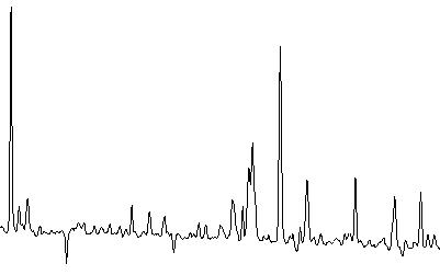
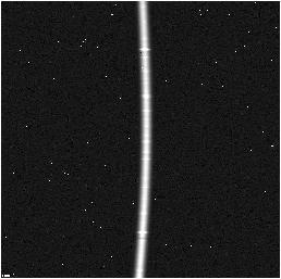
1) Frame with flat background and perpendicular trace
This is the most basic case. First load the FITS file into data:
IDL> frame1 = readfits('ex1.fits', header1)
Next, locate the read noise and gain levels for the CCD array. This
FITS file contains that information in the header.
IDL> Q = sxpar(header1, 'EPADU')
IDL> rn = sxpar(header1, 'RDNOISE') / Q
Now we need to select the object spectrum limits. This can be done
interactively using a plot of the frame. The trace is perpendicular,
any row will do.
IDL> plot, frame1[*,0]
IDL> plot, frame1[200:300,0]
It seems the spectrum spans columns 240 to 270.
IDL> x1 = 240
IDL> x2 = 270
Now we need to prepare the data and variance images. Since there is
no sky frame, the data image is the object frame. The inital estimate
for the variance image is easily calculated.
IDL> dataim = frame1
IDL> varim = abs(frame1) / Q + rn^2
With all of the data now prepared, run optspecextr.
IDL> opspec1 = optspecextr(dataim, varim, rn, Q, x1, x2)
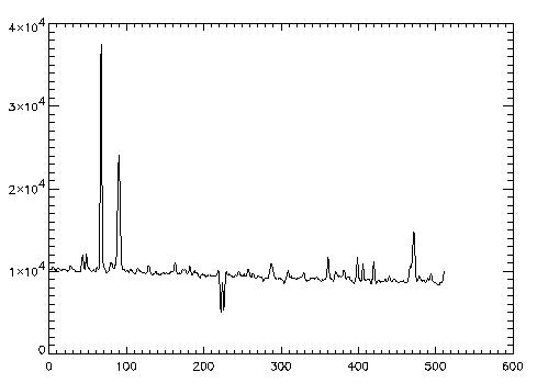
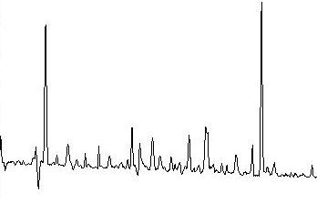
IDL> plot, opspec1
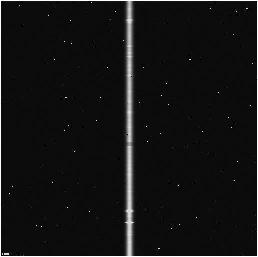
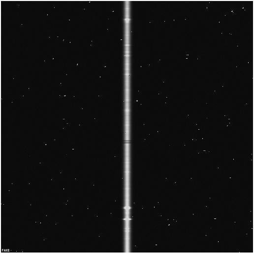
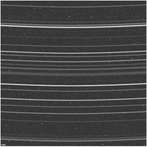
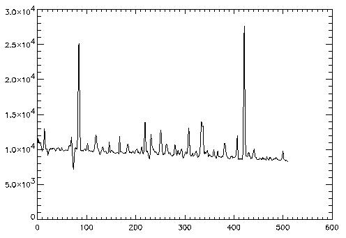
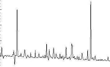
Object frame and extracted spectrum from a simple frame
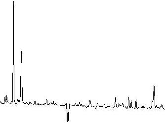
	2) Object and Sky frame

	When working with IR data and a sky frame is to be used for sky
	subtraction, that information needs to be passed onto the optimal
	extraction procedure.

	The preperation is identical to example 1.
	IDL> objframe2 = readfits('ex2obj.fits', objheader2)
	IDL> skyframe2 = readfits('ex2sky.fits', skyheader2)
	IDL> Q =     sxpar(objheader2, 'EPADU')
	IDL> rn =    sxpar(objheader2, 'RDNOISE') / Q
	IDL> rnsky = sxpar(skyheader2, 'RDNOISE') / Q
	IDL> x1 =    240
	IDL> x2 =    270

	The data image is object frame - sky frame.  An additional sky
	variance image must also be created.  The initial variance estimate
	must reflect the additional image processing step.
	IDL> dataim =   objframe2 - skyframe2
	IDL> skyvarim = abs(skyframe) / Q + rnsky^2
	IDL> varim =    abs(skyframe + objframe) / Q + rnsky^2 + rn^2

	The call for optspecextr uses the SKYVARIM keyword.
	IDL> opspec2 = optspecextr(dataim, varim, rn, Q, x1, x2, $
	                           skyvarim=skyvarim)
	IDL> plot, opspec2
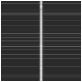
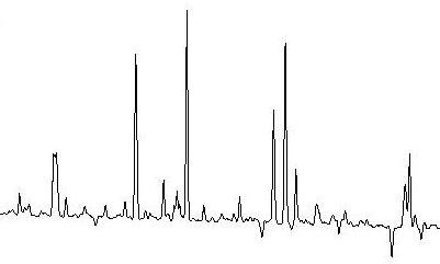
Object and sky frames, with resulting plot
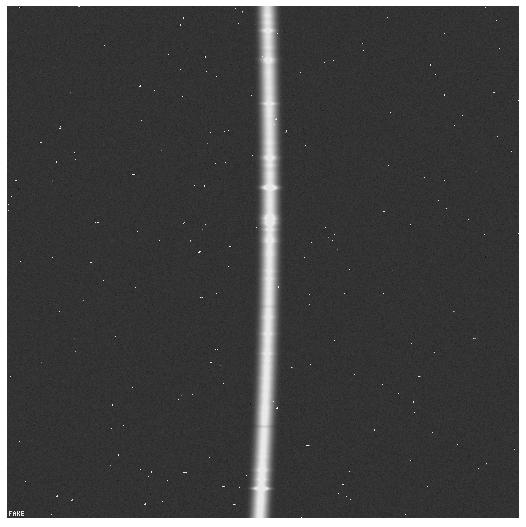
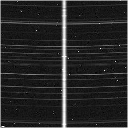
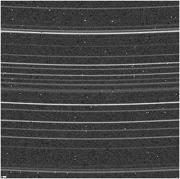
3) Frame with curved trace
A frame with a curved trace can not fit the profile using a polynomial
fit along the wavelength dimension because the profile changes to
quickly. Instead try either the boxcar filter, or gaussian fit.
The preperation begins the same.
IDL> frame3 = readfits('ex3.fits', header3)
IDL> Q = sxpar(header3, 'EPADU')
IDL> rn = sxpar(header3, 'RDNOISE') / Q
However, the curved trace makes setting spectrum limits more
difficult. Take a look at the frame to get the general idea.
IDL> tv, frame3
The minimum occurs and the top and bottom of the frame, while the
maximum occurs about halfway down the frame.
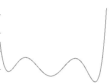
IDL> plot, frame3[200:300,0]
IDL> plot, frame3[200:300,255]
IDL> plot, frame3[200:300,511]
It seems to span from 240 to 280
IDL> x1 = 240
IDL> x2 = 280
Now run optspecextr with either the FITGAUSS or FITBOXCAR keyword.
IDL> dataim = frame3
IDL> varim = abs(frame3) / Q + rn^2
IDL> opspec3gauss = optspecextr(dataim, varim, rn, Q, x1, x2, $
/fitgauss)
IDL> dataim = frame3
IDL> varim = abs(frame3) / Q + rn^2
IDL> opspec3rsa = optspecextr(dataim, varim, rn, Q, x1, x2, $
/fitboxcar)
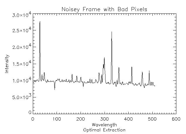
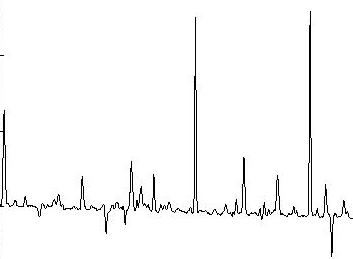
Exctraction using FITGAUSS and FITRSA repsectfully
	4) Straightening

	A curved frame may also be corrected using the STRAIGHTEN keyword.
        This technique upsamples the data frame by 10 pixels, shifts each
        row by an estimated center correction.  Then the usual fitting methods
        can be used to fit the expanded data.  Before use the profile is
        downsampled.

	The preperation begins the same.
	IDL> frame4 = readfits('ex4.fits', header4)
	IDL> Q =  sxpar(header4, 'EPADU')
	IDL> rn = sxpar(header4, 'RDNOISE') / Q

	In order to show the correction more clearly this frame is only curved
	in the x direction.  The shift4.fits file contains the shift amount
	IDL> traceact = readfits('shift4.fits')
        IDL> plot, traceact

	It seems to span from 235 to 270
	IDL> x1 = 235
	IDL> x2 = 270

	Now run optspecextr with the straighten keyword.  The TRACEEST keyword
	return the estimated shift amount.  With the expantion, straightening
	may take much longer than other techniques.
	IDL> dataim = frame4
	IDL> varim = abs(frame4) / Q + rn^2
	IDL> opspec4 = optspecextr(dataim, varim, rn, Q, x1, x2, $
	                           /straighten, traceest=traceest)

        IDL> plot, traceest
        IDL> plot, (traceest - 4) - traceact
Comparison between actual center shift and estmated
DEBUGGING ASSISTANCE:
        If the program does not work as expected the routine has specific
        keywords designed to assist in debugging.

        The VERBOSE keyword controls the level of output to the user.  By
        default it displays only fatal errors. With the level at 1, it will
        collect stats on the execution of the program, and if neccissary
        outputs them on a single line at the conclusion.  If VERBOSE is set to
        level 2, it will update the user on its location throughout the
        program.  Setting VERBOSE to 3 will give you warnings as the program
        believes the data is not acting according to plan.

        With VERBOSE at 4 the program will attempt to plot the data as it
        executes.  The PLOTTYPE keyword controls what type of plot to use.  1
        will plot shaded surfaces of the raw data about to be processed and
        the fitted data recently analyzed.  PLOTTYPE at 2 will give a summary
        of each vector before processing, and PLOTTYPE 3 will plot each
        iteration of cosmic ray identification.

        Setting VERBOSE to 5 keyword stops the exectution during the
        background fitting and profile fitting sections of the algorithm.  The
        keyword stops exectution right before entering the procvect routine
        (which actually does the fitting) and triggers procvect to stop after
        every iteration of the fit. The when stopped, the idl ".continue" or
        ".c" will continue execution until the next stop is encountered.
        When verbose is at 5 it will plot both PLOTTYPE 2 and 3 plots.


FAQ:
        1) Q: Why is everything in double precision when the input data is
	most likely single precision?

	A: The short answer is it prevents a systematic bias is the final
	output.  The cause of this bias was traced to an error in floating
	point representation of the profile image.  When a perfect (no noise,
	straight trace, no bad pixels, ...) image was tested, there was
	symetric error at machine level precision in the profile image created
	by looping procvect.pro.  However, as this image was scaled to make
	sure each wavelength summed to 1, the error became off-center.  This
	error was componded in later steps and eventually showed up in the
	final spectrum.  There was no way to scale a floating point array
	without this occuring, so instead everything is done in double
	precision.

	2) Q: Help! The program keeps masking all of my data points. What's
	wrong?

	A: The probable answer lies in the variance image creation.  The
	routine uses and iterative sigma-cliping calculation using:
	  Residual = (Data - Background - Spectrum*Profile)^2 / Variance
	If the variance estimate is wrong, the procvect routine can end up
	clipping way too many or too few pixels easily.  The background fiting
	and the first pass of the profile fitting use the inital variance
	estimates that are passed in.  However, each subsequent pass in
	profile fitting, and in the optimal extraction iteration, the variance
	image used is recalculated based on:
	  Variance = Readnoise^2 + Abs(Spectrum*Profile + Background) / EPADU
	Therefore, if your estimates for read noise or gain are off, each
	revisted estimate will be inaccurate.  The sigma-clipping routine is
	sensitve to both rdnoise and gain. If background pixels are wrongly
	masked, the readnoise is proabably off.  If the high-intensity pixels
	are masked, then it is probably the gain.

	Another problem could stem from inaccurate estimation of the fit.  If
	the profile image is changing more rapidly than can be modeled by a
	third degree polynomial, the degree must be increased, or a different
	fit used.  Similarly, if skylines are curved too much (more than three
	pixels spell distator for polynomial fitting) the background fitting
	routine won't be able to model the background.