Defringeflat
Version 1.4.1 (September 14th, 2005)
Patricio Rojo, Joseph Harrington (Cornell University)
Documentation
This routine removes a fringe pattern with repetitive
characteristics from a flat field.
Fringe Pattern
A typical flat field array from a VLT observation using the ISAAC
instrument is shown in Figure 1. In the
upper frame a periodic fringe pattern is clearly visible. It can also be
seen that the periodicity is not constant throughout the array but it
changes visibly, for example, in the upper right quadrant.
This change in periodicity gets confirmed in the lower frame of
figure 1 where only shortwards of pixel ~400 averaging brings up the
signal-to-noise, and longwards of that same pixel the average gets
flatten because the fringe period changes in that region.
Also, the smooth change in period inmediately explains while you
cannot use methods like Fast Fourier Transform (FFT) where only one
frequency per row can be found.
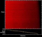 Figure 1: Upper frame is ISAAC's flat field image obtained after
subtraction of dark frame with same exposure time. Lower frame is
the average of every row.
Template id 'ISAACSW_spec_cal_NightCalib'. Integration time: '4
seg'. FITS file 'flat.fits' is supplied with defringeflat package.
Figure 1: Upper frame is ISAAC's flat field image obtained after
subtraction of dark frame with same exposure time. Lower frame is
the average of every row.
Template id 'ISAACSW_spec_cal_NightCalib'. Integration time: '4
seg'. FITS file 'flat.fits' is supplied with defringeflat package.
Wavelet
A more detailed, quantitative introduction to the wavelet transform
is given by C. Torrence and
G. Compo, only a brief introduction is presented below.
In short, the wavelet transform calculates the frequency spectrum in
a region around each point of a one-dimensional array, to give the
spectrum's variation with location in the array.
The size of the region scales with period, which is the main difference
from the windowed Fourier transform.
Figure 2 shows an example of a periodic
function (a sine function whose period changes linearly from 70 to 40
pixels) and its wavelet transform. The lower frame shows the amplitude
of the wavelet transform. The region in the shaded area is inside the
"cone of influence" of the edges of the data, which signals that these
values cannot be trusted.
A trace in the transform that peaks at the expected frequency is
clearly visible. However, this trace has a shape with some
non-zero width. As can be seen in cross-section (Figure 3), the shape is not quite a Gaussian, but it
gives a fair approximation.
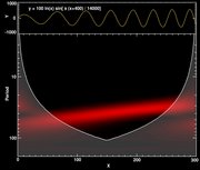 Figure 2. Upper frame: sinusoidal function whose period and
amplitude change from left to right. Lower frame: amplitude of
a Morlet wavelet transform of the spectrum.
Figure 2. Upper frame: sinusoidal function whose period and
amplitude change from left to right. Lower frame: amplitude of
a Morlet wavelet transform of the spectrum.
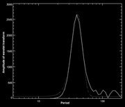 Figure 3. Vertical cross section of the wavelet transform's
amplitude (solid line) and the best-fit Gaussian (dotted line).
Figure 3. Vertical cross section of the wavelet transform's
amplitude (solid line) and the best-fit Gaussian (dotted line).
Fringe Calculation
Algorithm
The routine defringeflat uses the following procedure to compute the
fringe pattern of a flat field.
To improve the signal-to-noise ratio and remove "wild" pixels, a 1-D
median average of a specified number of rows is computed for each of the
rows (Figure 4).
For each of the filtered rows, the slope is subtracted through a linear
fit inside the specified trim limits, every point outside the
trim limits is replaced with zeroes, a wavelet transform is
performed according to specified wavelet parameters, and then possibly
interpolated (Figure 5).
We then identify the trace of the wavelet amplitudes that corresponds
to the fringe system. A specified function (see next section: Trace
fitting methods) is fit
to the trace profile using a user-identified fringe period (at some
reference image coordinates) as the initial guess (Figure 6). Then we follow the local maximum along the
columns. Repeating this procedure for each row, we obtain a fitted set
of parameters (e.g., center, width, and amplitude of a Gaussian) for
each pixel in the array.
If specified, each parameter array is compared to a median-filtered
version of itself to identify and replace outliers, and then
mean-smoothed (Figure 7).
Then, the wavelet transform is reconstructed from the
(smoothed) parameters obtaining the fringe's wavelet transform(Figure 8). Finally, an inverse wavelet transform is
performed to obtain the computed fringe pattern (Figure
9), which is then removed from the flat(Figure
10).
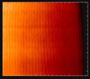 Figure 4. Flat field in Fig. 1 after being median averaged in the
vertical direction. In this particular example, each row is the median
average of the 40 rows surrounding it.
Figure 4. Flat field in Fig. 1 after being median averaged in the
vertical direction. In this particular example, each row is the median
average of the 40 rows surrounding it.
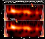 Figure 5. Upper frame shows middle row of Fig. 4. Middle frame shows the
amplitude of the wavelet transform in the relevant periods. Lower
frame: Same as middle frame but interpolated in period to 10 times the
original period resolution.
Figure 5. Upper frame shows middle row of Fig. 4. Middle frame shows the
amplitude of the wavelet transform in the relevant periods. Lower
frame: Same as middle frame but interpolated in period to 10 times the
original period resolution.
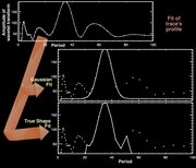 Figure 6. Cross section of wavelet transform's middle column, original
points are always represented by small crosses. Upper frame shows
original points and the interpolated profile (solid line). Middle and
lower frames show the profiles fitted (solid line) when using methods
'Gaussian' and 'true shape', respectively.
Figure 6. Cross section of wavelet transform's middle column, original
points are always represented by small crosses. Upper frame shows
original points and the interpolated profile (solid line). Middle and
lower frames show the profiles fitted (solid line) when using methods
'Gaussian' and 'true shape', respectively.
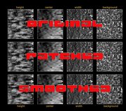 Figure 7. Parameter smoothing. From left to right the parameters
are amplitude, center, width, and background of a Gaussian fit of
the trace. From top to bottom, they are shown as raw
fitted, patched (bad pixels replaced), and smoothed parameters.
Figure 7. Parameter smoothing. From left to right the parameters
are amplitude, center, width, and background of a Gaussian fit of
the trace. From top to bottom, they are shown as raw
fitted, patched (bad pixels replaced), and smoothed parameters.
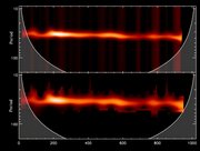 Figure 8. Fringe's wavelet. Amplitude of the reconstructed fringe
trace.
Figure 8. Fringe's wavelet. Amplitude of the reconstructed fringe
trace.
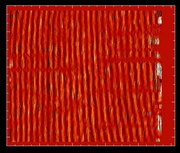 Figure 9. Fringe obtained from inverse transform of Figure 8.
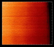 Figure 10. Flat field from Figure 1 after being cleaned by
defringeflat.
Figure 10. Flat field from Figure 1 after being cleaned by
defringeflat.
Trace Fitting Methods
Choosing the function to fit the cross-section of the wavelet's trace is
one of the most critical choices for a successfull cleaning. Therefore,
each of the alternatives of the keyword FITNAME is briefly explained
below.
- Gaussian (gauss): Default alternative. After
oversampling, a Gaussian function is fit to the trace's cross-section
(Middle frame in Figure 6). Four parameters (height, center, width,
background) are obtained and can be smoothed. Using this method
will not fit every wavelet point perfectly, but is more robust against
removing non-fringe patterns from the image.
- Gaussian Estimate (gaussest): Is similar to the above
Gaussian fit, but the parameters are only estimated. Height is
the highest value of the trace, center is the period of the
highest value, width is one-fifth (chosen arbitrarily as a good
approximation) of the separation between the local lower minima, and
background is zero. There is not really any advantage in
choosing this alternative instead of the above other than for speed or
as a failproof alternative.
- True shape (trueshape): Once the trace's peak has been
found, all the points between the local lower minima at the sides of the
trace (lower frame in Figure 6) are used to reconstruct the fringe's
wavelet. The main disadvantage of this approach is that every single
feature of the wavelet around the peak period is going to be removed
from the original image. This might include real features from the
image that were not intended to be cleaned. Smoothing of parameters is
not available.
Execution example
To run this example you would need the wavelet routines from C. Torrence and
G. Compo and the astrolib routines from NASA.
IDL> flat  = readfits('example/flat.fits', h)
IDL> func  = 'gauss'
IDL> clean = defringeflat(flat, 40, binw=40, trim=[10,145,950,950], $
		          osamp=10, /smooth, fitname=func, fringe=fringe)
IDL> tvscl, flat
IDL> tvscl, fringe
IDL> tvscl, clean
Error estimates
It is difficult to estimate the error given that the real shape of the
fringes is unknown. However, the effectiveness of this method can
be seen by how much does the fringe pattern disappear.
Let's take a look at the average of the rows from the VLT flat
field. As it was discussed regarding Fig. 1, in the
first third of the columns the period of the fringes remain constant,
and hence the average just increases the signal-to-noise ratio.
Figure 11 shows columns 30 to 250 of the average
of all rows before and after having the fringe pattern removed by
defringeflat routine using 'true shape' and Gaussian fitting
functions. It is visible to the naked eye as well as in their power
spectrum that the fringe pattern was fully removed. True shape seems to
remove more throughfully, but there is more risk that it is also
removing real flat fields artifacts.
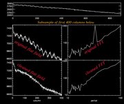 Figure 11: Fringe removal efficiency. Upper frame is original average of
rows. Upper left: Subsample of the first 400 columns of the plot in
Figure 1. Middle left: Same subsample after Gaussian fringe
cleaning. Lower left: Same subsample after 'true shape' fringe
cleaning. Right panels: FFT power spectra of data in corresponding left
panels.
Figure 11: Fringe removal efficiency. Upper frame is original average of
rows. Upper left: Subsample of the first 400 columns of the plot in
Figure 1. Middle left: Same subsample after Gaussian fringe
cleaning. Lower left: Same subsample after 'true shape' fringe
cleaning. Right panels: FFT power spectra of data in corresponding left
panels.
Acknowledgements
Work supported by the NASA Origins of Solar Systems program.
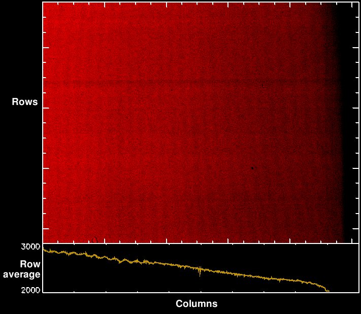 Figure 1: Upper frame is ISAAC's flat field image obtained after
subtraction of dark frame with same exposure time. Lower frame is
the average of every row.
Template id 'ISAACSW_spec_cal_NightCalib'. Integration time: '4
seg'. FITS file 'flat.fits' is supplied with defringeflat package.
Figure 1: Upper frame is ISAAC's flat field image obtained after
subtraction of dark frame with same exposure time. Lower frame is
the average of every row.
Template id 'ISAACSW_spec_cal_NightCalib'. Integration time: '4
seg'. FITS file 'flat.fits' is supplied with defringeflat package.
 Figure 2. Upper frame: sinusoidal function whose period and
amplitude change from left to right. Lower frame: amplitude of
a Morlet wavelet transform of the spectrum.
Figure 2. Upper frame: sinusoidal function whose period and
amplitude change from left to right. Lower frame: amplitude of
a Morlet wavelet transform of the spectrum. Figure 3. Vertical cross section of the wavelet transform's
amplitude (solid line) and the best-fit Gaussian (dotted line).
Figure 3. Vertical cross section of the wavelet transform's
amplitude (solid line) and the best-fit Gaussian (dotted line).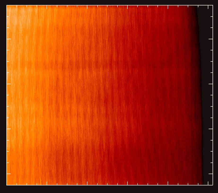 Figure 4. Flat field in Fig. 1 after being median averaged in the
vertical direction. In this particular example, each row is the median
average of the 40 rows surrounding it.
Figure 4. Flat field in Fig. 1 after being median averaged in the
vertical direction. In this particular example, each row is the median
average of the 40 rows surrounding it.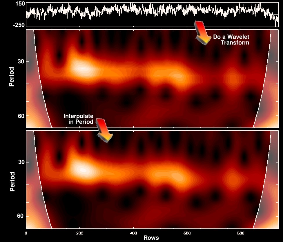 Figure 5. Upper frame shows middle row of Fig. 4. Middle frame shows the
amplitude of the wavelet transform in the relevant periods. Lower
frame: Same as middle frame but interpolated in period to 10 times the
original period resolution.
Figure 5. Upper frame shows middle row of Fig. 4. Middle frame shows the
amplitude of the wavelet transform in the relevant periods. Lower
frame: Same as middle frame but interpolated in period to 10 times the
original period resolution. Figure 6. Cross section of wavelet transform's middle column, original
points are always represented by small crosses. Upper frame shows
original points and the interpolated profile (solid line). Middle and
lower frames show the profiles fitted (solid line) when using methods
'Gaussian' and 'true shape', respectively.
Figure 6. Cross section of wavelet transform's middle column, original
points are always represented by small crosses. Upper frame shows
original points and the interpolated profile (solid line). Middle and
lower frames show the profiles fitted (solid line) when using methods
'Gaussian' and 'true shape', respectively. Figure 7. Parameter smoothing. From left to right the parameters
are amplitude, center, width, and background of a Gaussian fit of
the trace. From top to bottom, they are shown as raw
fitted, patched (bad pixels replaced), and smoothed parameters.
Figure 7. Parameter smoothing. From left to right the parameters
are amplitude, center, width, and background of a Gaussian fit of
the trace. From top to bottom, they are shown as raw
fitted, patched (bad pixels replaced), and smoothed parameters. Figure 8. Fringe's wavelet. Amplitude of the reconstructed fringe
trace.
Figure 8. Fringe's wavelet. Amplitude of the reconstructed fringe
trace. Figure 9. Fringe obtained from inverse transform of Figure 8.
 Figure 10. Flat field from Figure 1 after being cleaned by
defringeflat.
Figure 10. Flat field from Figure 1 after being cleaned by
defringeflat. Figure 11: Fringe removal efficiency. Upper frame is original average of
rows. Upper left: Subsample of the first 400 columns of the plot in
Figure 1. Middle left: Same subsample after Gaussian fringe
cleaning. Lower left: Same subsample after 'true shape' fringe
cleaning. Right panels: FFT power spectra of data in corresponding left
panels.
Figure 11: Fringe removal efficiency. Upper frame is original average of
rows. Upper left: Subsample of the first 400 columns of the plot in
Figure 1. Middle left: Same subsample after Gaussian fringe
cleaning. Lower left: Same subsample after 'true shape' fringe
cleaning. Right panels: FFT power spectra of data in corresponding left
panels.