1. Introduction

This Assignment extends the spreadsheet that you created in Assignment 1, to include numerical integration as well as numerical differentiation.

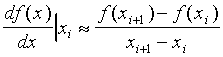
Consider a function f(x), which can be calculated by an explicit formula at a set of points x_i. In assignment No. 1 you made a spreadsheet that calculated and graphed the derivative of this function, using the approximation:

. [1]

This equation says that the value of the derivative (or slope) of the function f(x), at the point x_i, can be calculated from the difference in the value of the function at two nearby points.

A simple example of where you can use this formula is in the evaluation of the velocity of a particle, given its position as a function of time: dx(t)/dt = v(t).

It is also possible to find the position of a particle as a function of time, given the value of the velocity. This involves the integral:

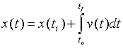. [2]

In this exercise you will use two different methods to calculate the integral using a spreadsheet: the Euler method and the ``half-step'' method. You will also solve the problem exactly, and compare the exact answer to the two approximations. You will start with an example spreadsheet and modify it see how things work.

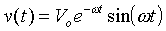
In this problem, let the velocity be given by v(t) = V_o sin(wt). The exact solution to Eq. 2 is:

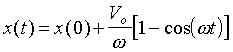. [3]

as you can easily check for yourself.

To solve this problem using the Euler method, we remember that an integral is just the area under a curve. In this case the curve is v(t). The Euler approximation is:

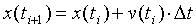. [4]

Here we see that we need to define a small step in time:

.

For the half-step method, we simply get the velocity at a time half-way between t_i and t_i+1=t_i+Dt. That is,

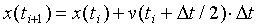. [5]

Although in this simple case, the two methods give similar answers, in general the half-step technique is a better way to calculate an integral.

2. Tasks

Examine the behavior of the position of the particle as a function of time graphically, and numerically. Calculate the position exactly and by using the numerical integration technique.

You should turn in the following solutions. In each case, print out a new copy of the first page of the spread-sheet, which contains the definitions and first few data points, as well as an annotated graph.

1. Calculate the motion for a frequency of w=2 Hz, and a time step size of Dt=0.05 sec. Put labels on your graph to show V_o, w, and Dt.
2. Repeat the exercise with different parameters of your choice.
3. Change the formula for the velocity to the following

.

Plot the motion of the particle with this new form for the velocity, which is similar to a particle on a spring with friction. Note that the ``exact'' column calculation no longer applies.